Free electrode occipital SSVEP montage¶

Eight free (unmounted) electrodes in a tight cluster over the occipital pole, wired to an OpenBCI Cyton, with reference and ground on the earlobes. "Free electrode" means the electrodes are placed individually on the scalp — gold cups with paste, or the lab's dry headband, which carries the same layout in a fixed carrier.

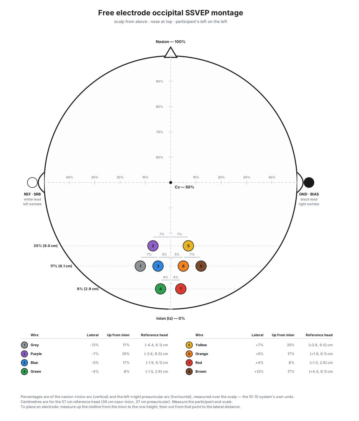
Positions are given as percentages of the participant's own head, in the same units the 10-10 system uses, but they are not 10-10 sites. See Occipital 10-10 montage for the standard-sites montage, which is the toolbox's default.

The montage, scalp seen from above

1. Why choose this over standard 10-10 sites¶

The 10-10 grid puts nothing between the midline and PO3. Over the occipital pole — where the SSVEP is largest — the nearest off-midline sites a standard montage can use sit 7.6–9.7 % of the preauricular arc out, and there is no standard site closer in. This layout puts four channels at 4–5 %, in the gap the grid leaves empty, and still keeps a pair at 12 % further out. Two pairs of its channels are nearest to the same standard site (§5), which is the clearest statement of how much denser it is than the grid can be.

That is the whole case, and it is worth weighing against what it costs:

The channels have no standard names. They are wire colours. A reader — or an analysis pipeline — cannot tell what Orange is without this document.
Nobody else has it. Reproducing the montage means reading §2 and measuring, rather than reaching for a cap.
Nothing lines up with the literature. Reported SSVEP amplitudes at Oz or PO3 are not directly comparable to a channel that is merely near them.

Use this montage when the goal is the best occipital SSVEP that eight free electrodes can give and the comparison is internal — including any comparison against the lab's existing pilot data, which was collected on it. Use the 10-10 montage when the result is meant to be published or compared with other labs, when a cap is available, or when a reader needs to know what a channel is without reading a montage doc.

Nothing stops a study from running both; the carrier is recorded per session, so a sidecar always says which was on the participant's head.

2. The montage is defined in 10-10 units, not centimetres¶

The layout began life as a set of tape-measure centimetres taken on one lab head — an internal drawing, not distributed with the toolbox: 6 cm up from the inion, then 4.5 cm left. That works exactly once — on a head the size of the one it was measured on. Head circumference in adults spans roughly 52–60 cm, so a fixed centimetre offset lands on a materially different piece of cortex from one participant to the next, and on a child it is not close.

The 10-10 system solves this by expressing every position as a percentage of the participant's own head, and this montage is now stated the same way:

Height — distance up from the inion, as a percentage of the nasion→inion arc measured over the scalp along the midline.
Lateral — distance out from the midline, as a percentage of the left→right preauricular arc measured over the scalp through Cz.

Those are the same two denominators that place Oz, POz and Pz, so a position stated this way means the same thing on any head, and the figures in this document can be checked against any 10-10 chart.

Ch	Wire	Lateral	Up from inion	57 cm head
1	Grey	−12 %	17 %	4.4 cm left, 6.1 cm up
2	Purple	−7 %	25 %	2.6 cm left, 9.0 cm up
3	Blue	−5 %	17 %	1.9 cm left, 6.1 cm up
4	Green	−4 %	8 %	1.5 cm left, 2.9 cm up
5	Yellow	+7 %	25 %	2.6 cm right, 9.0 cm up
6	Orange	+5 %	17 %	1.9 cm right, 6.1 cm up
7	Red	+4 %	8 %	1.5 cm right, 2.9 cm up
8	Brown	+12 %	17 %	4.4 cm right, 6.1 cm up

Negative lateral = participant's left. The three rows straddle Oz (8 %), sit between Oz and POz (17 %), and between POz and Pz (25 %).

The percentages are whole numbers on purpose. Converting the original centimetres exactly gave 12.16 / 6.76 / 5.41 / 4.05 % and 8.33 / 16.67 %, which is spurious precision twice over: it states to a tenth of a millimetre something that came off a tape measure, and nobody at the bench computes 6.76 % of a 37.4 cm arc. Rounding to whole percent moves every electrode by at most 1.5 mm — well inside how accurately a free electrode can be placed at all — and gives numbers an operator can do in their head.

Where the percentages came from¶

The original drawing was measured on a head taken to be 57 cm in circumference. At that size the nasion→inion arc is about 36 cm and the preauricular arc about 37 cm (the usual ≈0.63 and ≈0.65 of circumference). Dividing the original centimetres by those two arcs, then rounding to whole percent, gives the table above. This is a restatement of the existing montage, not a new one — tests/test_montage.py::test_percentages_stay_within_1_5_mm_of_the_original_centimetre_drawing holds the drift to 1.5 mm on the reference head, and fails if anyone widens it.

The 36 / 37 assumption is not free-floating: MNE's standard_1005 template head gives a ratio of 0.975 between the two arcs, against 36/37 = 0.973.

Scaling to a participant¶

Measure the two arcs on the participant with a tape, then multiply:

distance (cm) = percentage / 100 × that participant's arc length (cm)

ssvep.stim.builder.montage_pct_to_cm(lateral_pct, height_pct, nasion_inion_cm, preauricular_cm) does this. On a 52 cm head (naso-inion ≈ 32 cm, preauricular ≈ 33 cm) channel 1 lands 4.0 cm left and 5.4 cm up, not 4.4 and 6.1 — about 5–7 mm of difference on each axis, which at this spacing is most of the gap between two neighbouring electrodes.

3. Placing it¶

You need a flexible tape measure, a skin-marking pencil, and the three landmarks: nasion (the dip between the eyes, at the bridge of the nose), inion (the bump at the back of the skull, on the midline), and the two preauricular points (the notch just in front of each ear canal).

Measure the nasion→inion arc over the top of the head, passing through the midline. Write it down. Measure the left→right preauricular arc over the top, crossing the first at Cz. Write that down too.
Convert the table above to centimetres for this participant (percentage ÷ 100 × arc).
For each row, measure up the midline from the inion to the row's height and mark the midline point. Keep the tape in line with the nasion so the measurement stays centred.
From that mark, measure out to each side to the lateral distance and mark the electrode position. Lay the tape flat on the scalp — the measurement follows the curve of the head, not a straight line through the air.
Part the hair, prep the site, and place the electrode. Match each electrode to its position by wire colour (§4) — on a free-electrode array the colour is the only thing telling one electrode from another.

The montage in place, head from behind

Reference and ground go on the ears¶

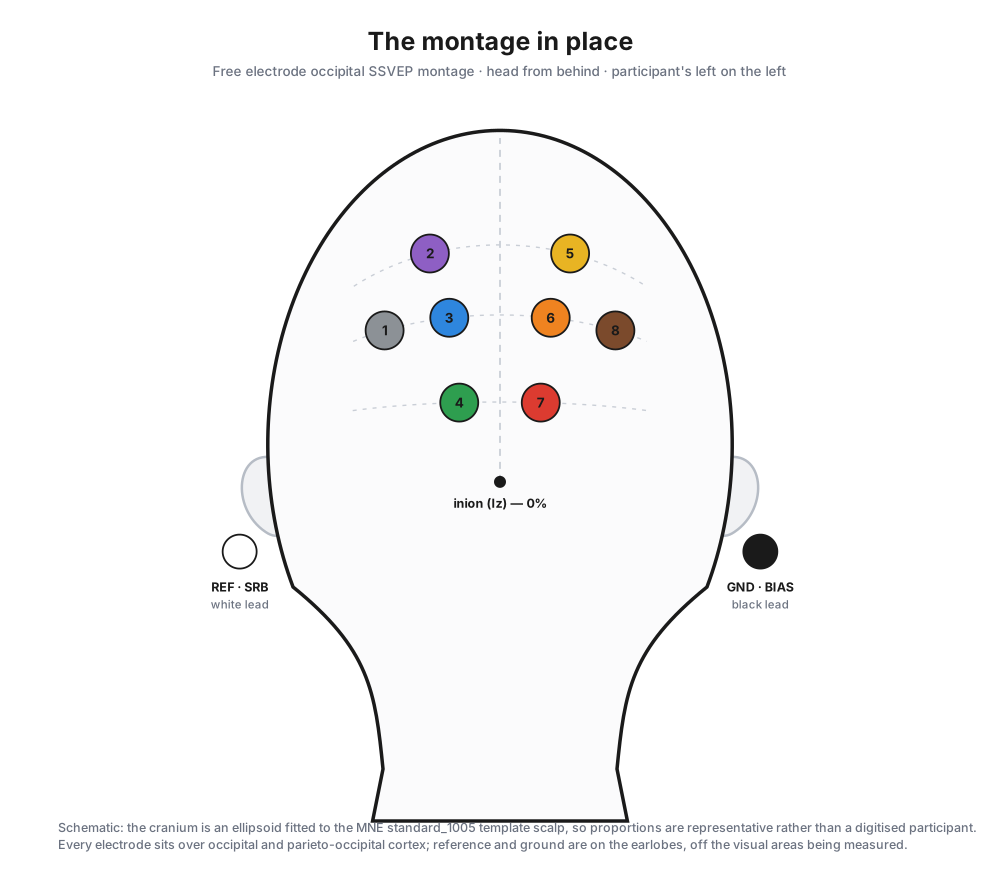
Reference — the white lead, Cyton SRB — on the LEFT earlobe (A1).
Ground — the black lead, Cyton BIAS — on the RIGHT earlobe (A2).

Both are off the visual cortex, so neither carries much of the SSVEP being measured, and an earlobe can be placed identically on every participant without a measurement.

This is the opposite of the original drawing

The original centimetre drawing this montage descends from puts GND and REF on the scalp, in the top row, and labels the left side GND and the right REF. Both of those are superseded: reference and ground are on the ears, and it is reference on the left, ground on the right. Recordings made before this change name a scalp reference in their sidecar; read them as they are recorded, not as this document describes.

4. Wiring the Cyton¶

Channel colours follow OpenBCI's standard Cyton ribbon-cable order — 1 grey, 2 purple, 3 blue, 4 green, 5 yellow, 6 orange, 7 red, 8 brown. This is the board's convention, not the lab's: anyone who has wired a Cyton already knows it, and it is what the OpenBCI documentation shows.

Pin	Wire	Goes to
`N1P`	Grey	ch1 — 12 % left, 17 % up
`N2P`	Purple	ch2 — 7 % left, 25 % up
`N3P`	Blue	ch3 — 5 % left, 17 % up
`N4P`	Green	ch4 — 4 % left, 8 % up
`N5P`	Yellow	ch5 — 7 % right, 25 % up
`N6P`	Orange	ch6 — 5 % right, 17 % up
`N7P`	Red	ch7 — 4 % right, 8 % up
`N8P`	Brown	ch8 — 12 % right, 17 % up
`SRB`	White	reference — left earlobe (A1)
`BIAS`	Black	ground — right earlobe (A2)
`AGND`	—	analogue ground; nothing connects to it

Cyton connections

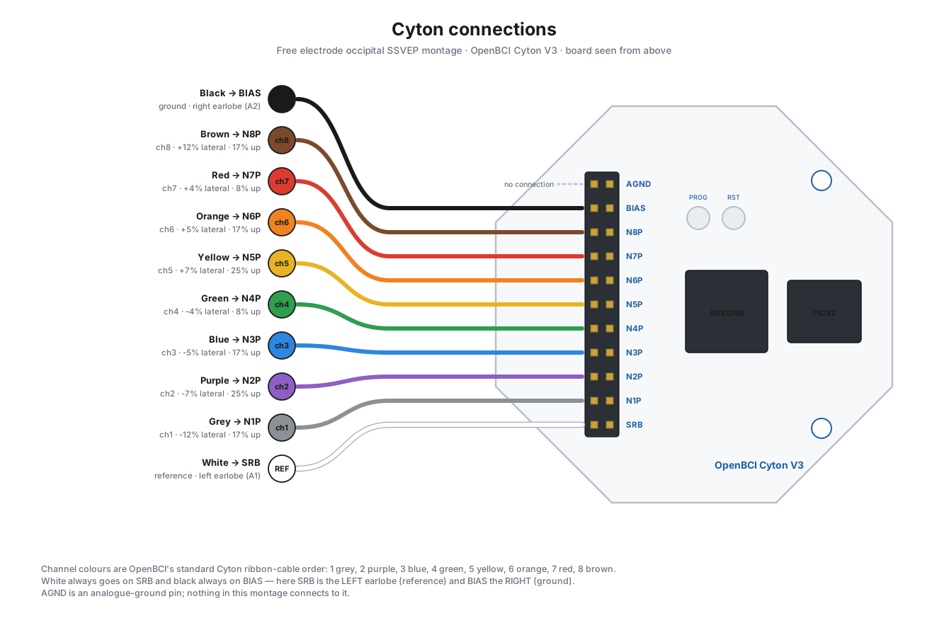
The eleven-pin header runs AGND, BIAS, N8P … N1P, SRB from one end to the other, so N1P is at the far end next to SRB. The board also silkscreens AVDD above the header and AVSS below it; those label separate two-pin sockets rather than positions on this header, and nothing here connects to them.

The reference pin is silkscreened SRB — one name, the one printed on the board you are holding. The header is a double row and we always use the row nearer the board, so the SRB1/SRB2 distinction in the ADS1299 datasheet never has to be made. Reference photo: OpenBCI's EEG setup page.

5. Where it sits relative to the 10-10 system¶

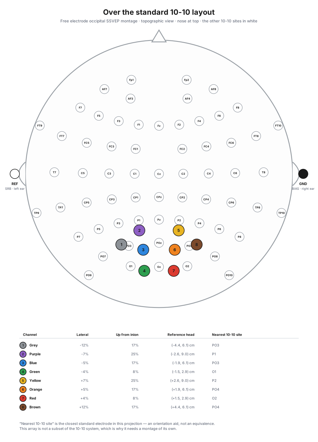
The montage over a standard 64-channel 10-10 layout

The array is not a subset of the 10-10 system — that is the whole reason it needs a montage of its own. The nearest standard sites are a rough orientation aid only:

Ch	Nearest 10-10 site
1 Grey	PO3
2 Purple	P1
3 Blue	PO3
4 Green	O1
5 Yellow	P2
6 Orange	PO4
7 Red	O2
8 Brown	PO4

Because the channels carry colour names rather than 10-10 labels, the decoder treats this montage as "already occipital" and uses every channel — see ssvep.spatial, which keys that decision off the declared montage size rather than off what a channel happens to be called. (A name-based heuristic once selected "Orange" as an occipital channel because it starts with "O".)

6. How the montage reaches the toolbox¶

The percentage table is the single source of truth, in ssvep.stim.builder.OCCIPITAL_SSVEP_MONTAGE_PCT. Everything else is derived from it:

Thing	Where
The montage	`builder.occipital_ssvep_montage()`
Carrier name	`builder.FREE_ELECTRODE_HEADSET`
Same layout, dry electrodes	`builder.ZEIST_HEADSET`
Wire colours	`builder.CYTON_CHANNEL_WIRE_COLOURS`
Reference / ground strings	`builder.OCCIPITAL_SSVEP_REFERENCE` / `..._GROUND`
Reference / ground for a carrier	`builder.headset_reference_ground()`
Reference head	`builder.REFERENCE_HEAD_CIRCUMFERENCE_CM` and the two arc constants
Percentage → cm	`builder.montage_pct_to_cm()`

In a recorded manifest, each montage channel carries both forms:

{ "channel": "E1", "label": "Grey",
  "position_pct": [-12, 17],
  "position_2d":  [-4.44, 6.12] }

position_pct is the definition — head-size independent, so it says where the electrode goes on any head. position_2d is the same point in centimetres on the reference head, and is what the discrete channel-array plots (the impedance map, the topographies) lay out. Fixed-geometry carriers — the g.tec Unicorn, the actiCAPs — have no position_pct: their electrodes are moulded in or held in a cap, so there is no tape-measure definition to record. Neither does the 10-10 montage, for a different reason: its site names already say where the electrodes go.

Carrier names recorded before September 2026¶

The carrier used to be listed under two other names, and every protocol and sidecar already on disk still says one of them. Both still resolve, one-way — nothing writes them back out:

Recorded name	Resolves to
`OpenBCI 8-ch occipital (default)`	`Free electrode occipital SSVEP montage`
`Free electrodes (gold-cup + paste)`	`Free electrode occipital SSVEP montage`

builder.canonical_headset() does the mapping; an unrecognised carrier passes through unchanged, because an unknown name is data to preserve rather than an error to raise.

7. Regenerating the figures¶

The four SVGs in docs/figures/montage/ are generated, not drawn. One run produces the figures for every montage the toolbox ships:

python scripts/build_montage_figures.py

A figure drawn by hand would be a second copy of the percentage table, and the second copy is the one that goes stale. tests/test_montage.py::test_figures_are_up_to_date_with_the_montages re-runs the script and fails if any figure changes — so a montage edit that nobody re-rendered is caught before it ships.

Figures 3 and 4 need an actual head to draw on, so the percentage walk is done as a geodesic on an ellipsoid fitted to MNE's standard_1005 template scalp: a tape laid flat on a head follows the shortest path over the surface, which is what a geodesic is. The fitted ellipsoid and the projected 10-10 coordinates are baked into the script as constants, so it needs nothing but numpy — mne was used once, at authoring time, and is not a dependency.